Analyzing Geo-spatial Data

In this tutorial, we will discuss analyzing geo-spatial data sources: specifically, we will explore conducting image segmentation tasks over satellite and aerial imagery. For example, we may wish to develop an ML pipeline for identifying oil drilling pad sites in satellite imagery.

Annotating Imagery

The first step is to obtain some labeled data. Here, we assume we want to annotate data in SkyhookML, but existing data in GeoJSON format can easily be imported as well.

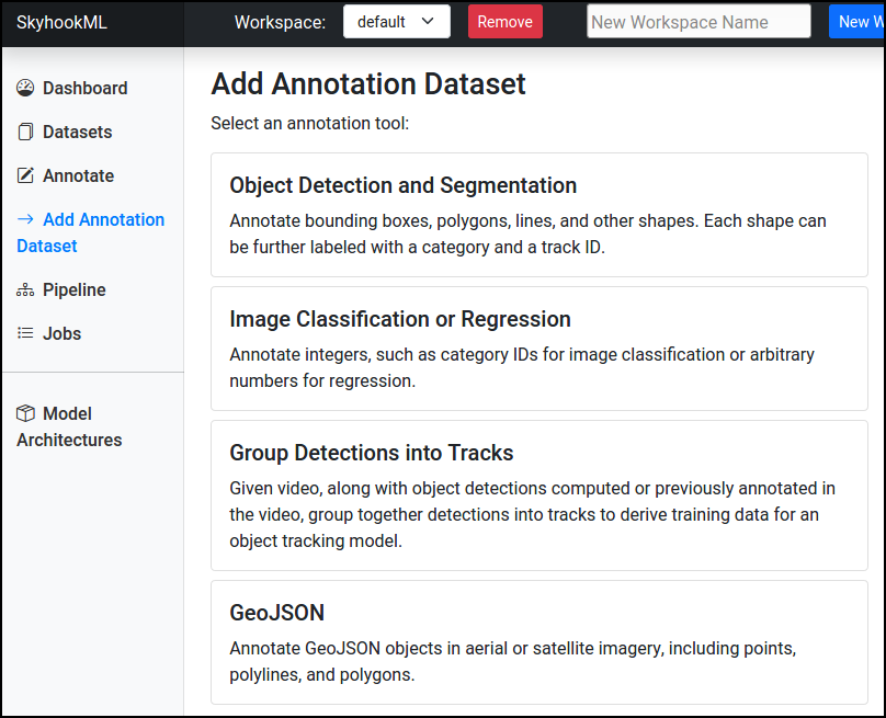
Go to the Dashboard, and select Annotate from the Quickstart options. For our task, we want to annotate GeoJSON objects:

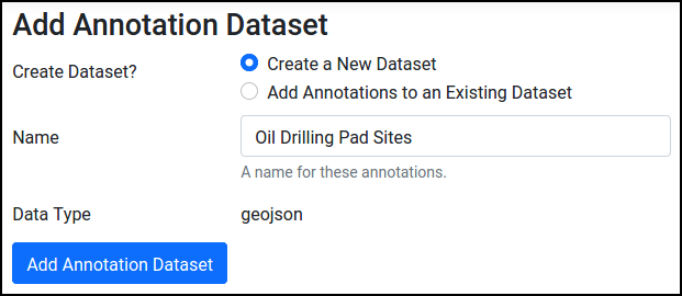
Give the annotation dataset a name, and create it:

This should load a mostly blank page asking for a Tile URL. This must be configured with a web endpoint that serves Web-Mercator imagery tiles. For example, for ESRI World Imagery, use https://services.arcgisonline.com/arcgis/rest/services/World_Imagery/MapServer/tile/{z}/{y}/{x}. After entering the Tile URL, press Save Settings.

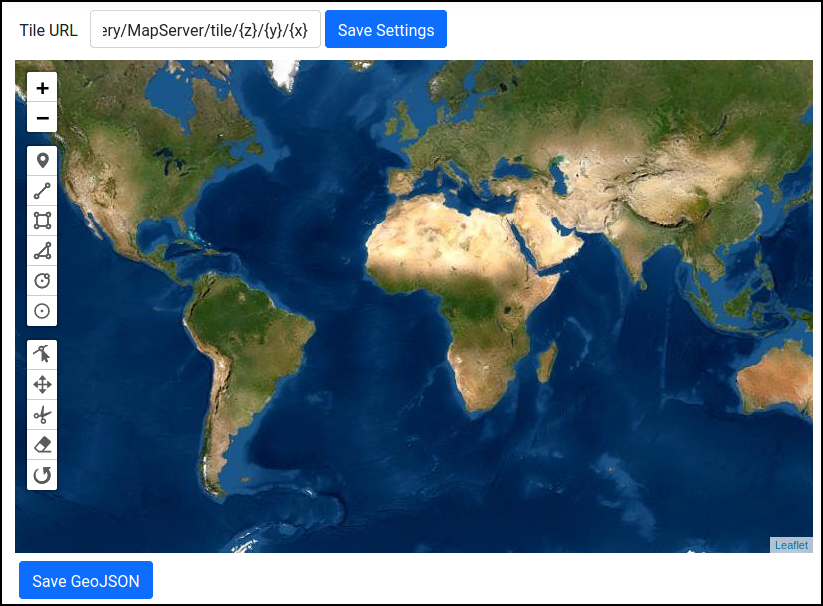
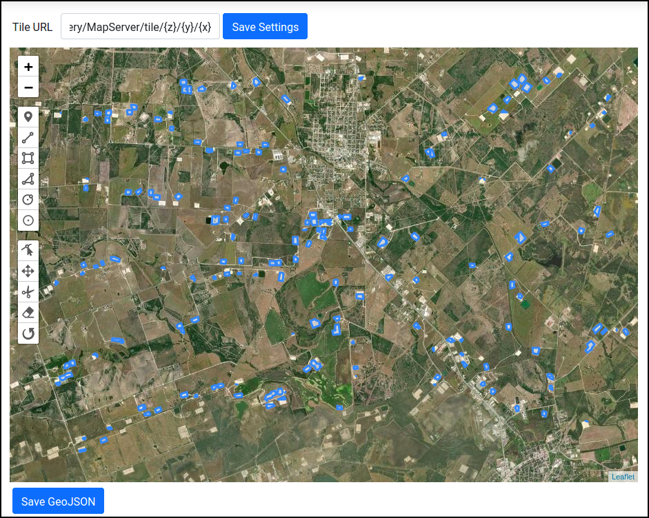
The buttons in the left sidebar panel can be used to label various types of features, including points, polylines, rectangles, and polygons. For example, we could label polygons around oil drilling pad sites visible in the ESRI World Imagery layer:

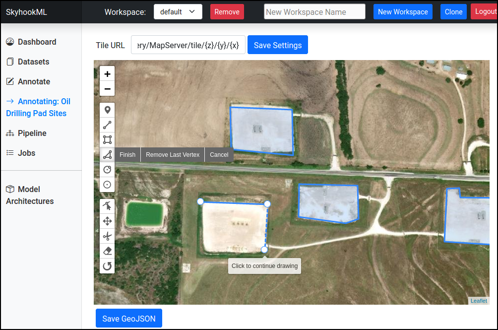
When done annotating GeoJSON features, press the Save GeoJSON button at the bottom to ensure that the features are saved into the GeoJSON dataset in SkyhookML.

Pre-processing

Before training a model on our labels, we need to perform several pre-processing steps, including:

Download windows of imagery around the GeoJSON features we annotated.
Convert the GeoJSON features to segmentation masks.

Let's first download the images. From Pipeline, press Add Node to create a Make Geo-Image Dataset operation:

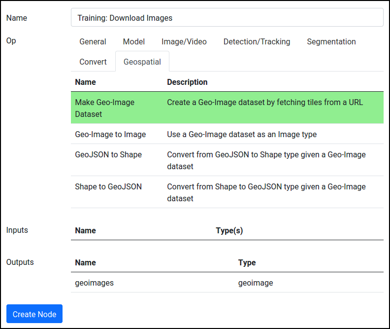
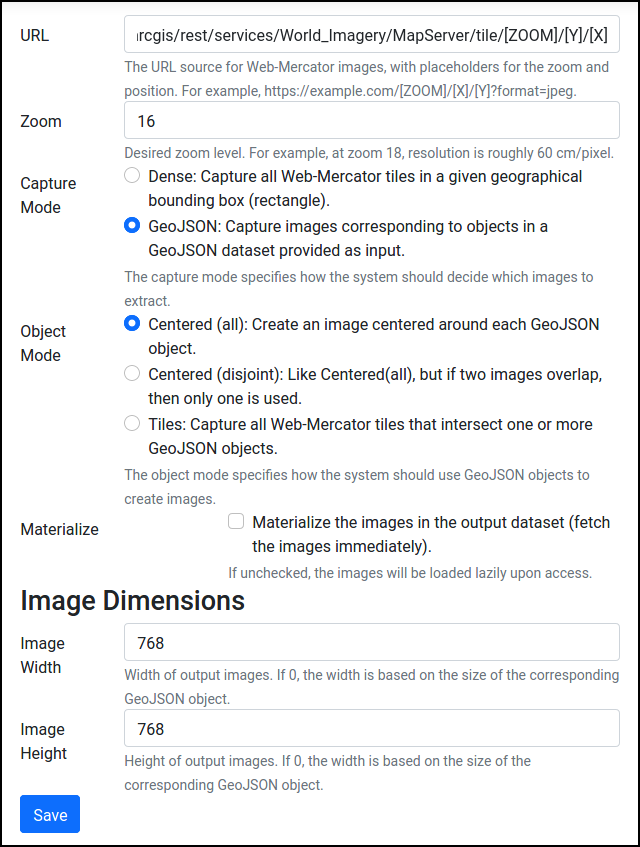
After creating the node, Edit it. We'll need to fill in a few options, such as the URL serving Web-Mercator tiles (e.g., https://services.arcgisonline.com/arcgis/rest/services/World_Imagery/MapServer/tile/[ZOOM]/[Y]/[X]), and how we want to decide which images to capture. For the oil site task, we opt to create a 768x768 image centered around each polygon that we labeled.

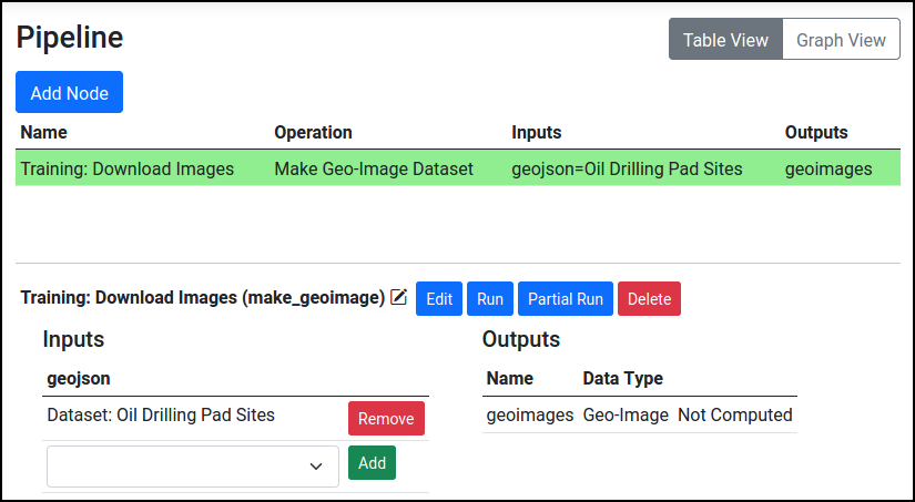
Once the node is configured, if using the GeoJSON capture mode, make sure to provide it with the GeoJSON annotations dataset as input:

Finally, add a "Geo-Image to Image" node that converts the Geo-Image dataset produced by the Make Geo-Image Dataset operation into an Image dataset. Edit this operation so that the Materialize option is set.

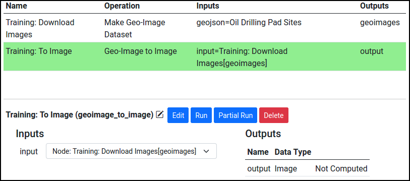
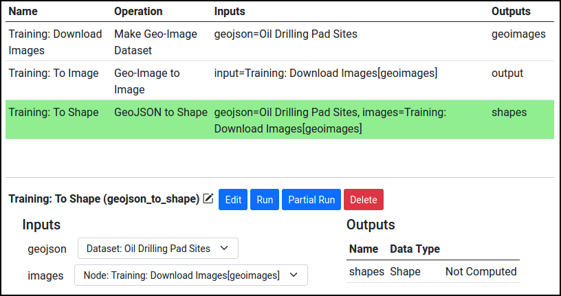
Now, let's produce segmentation masks so we can actually train an image segmentation model. We need to first convert our features from GeoJSON (longitude-latitude coordinates) to Shapes (pixel coordinates corresponding to our extracted images), and then produce masks from the shapes. Add a GeoJSON to Shape operation, and configure it so that it inputs the GeoJSON annotations along with the Geo-Images produced by the Make Geo-Image Dataset operation:

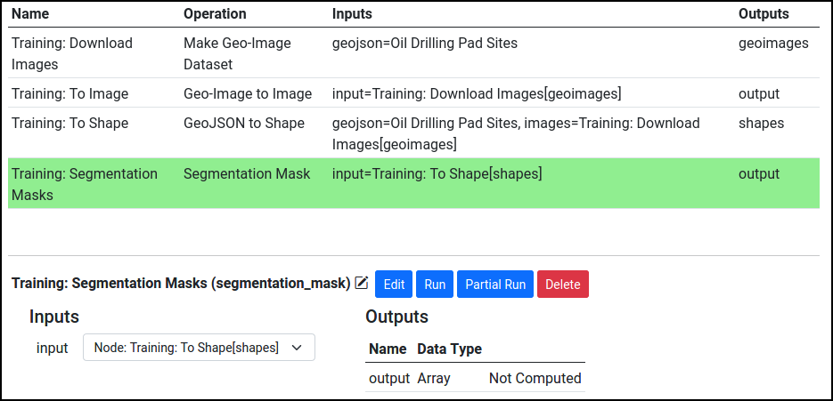
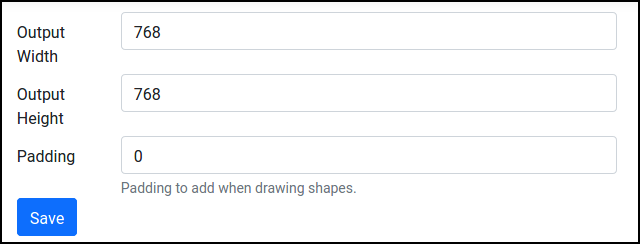
Then, add a Segmentation Mask node (from Segmentation tab) to create segmentation masks from shapes. This should input the shapes produced by the GeoJSON to Shape operation. Make sure to edit this operation and set the output width and height equal to the width and height of the downloaded images.

Training

We can finally train our image segmentation model! Add a UNet (train) node to the pipeline. It should input the converted images, along with the produced segmentation masks:

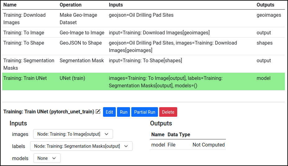
The train node can be edited to set desired training parameters, although the defaults should be sufficient. This trains a UNet segmentation model, which consists of an encoder with strided convolutional layers, a decoder with strided transpose convolution layers, along with skip connections between the two. Then, train the model!

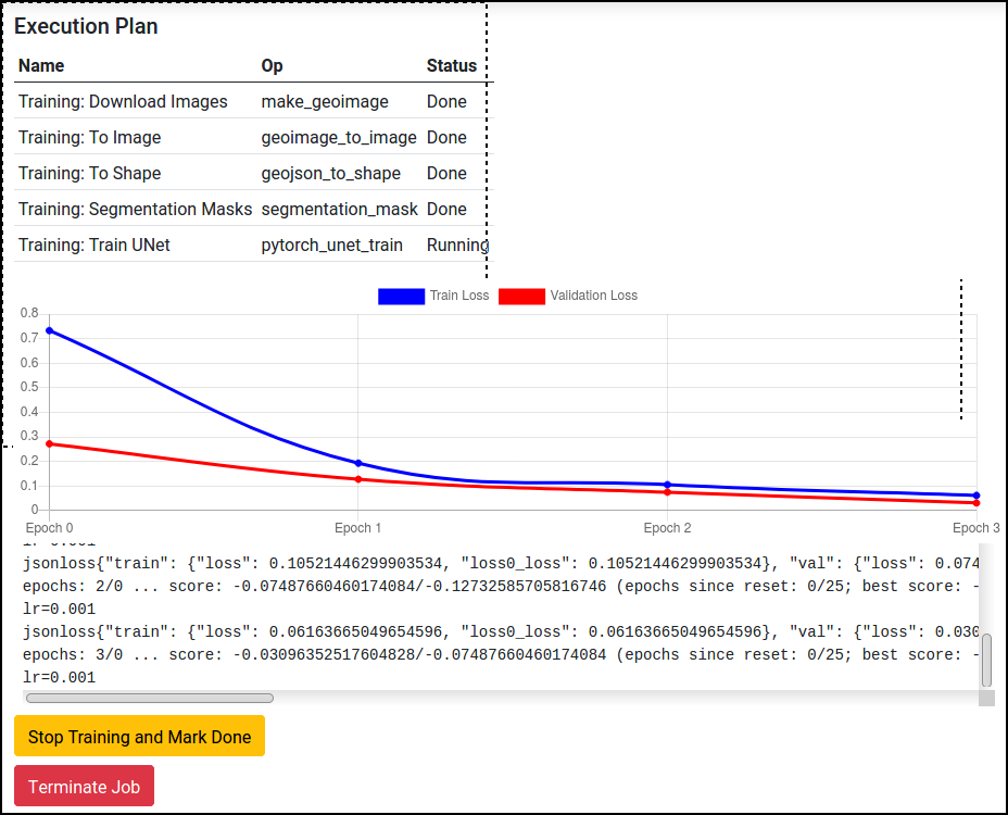
Inference

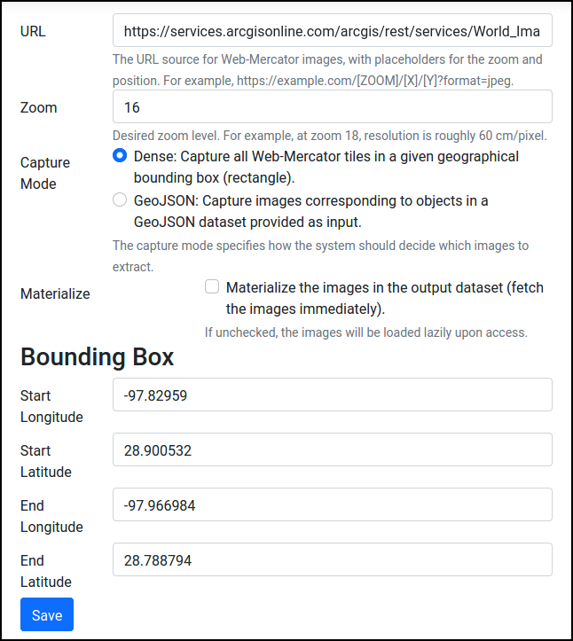
To apply our model for inference, we first need to download more images to run the model on. To do so, we can add another Make Geo-Image Dataset node. This time, for our example, we opt to download all images in a bounding box. Again, another node is needed to convert the Geo-Images into Images.

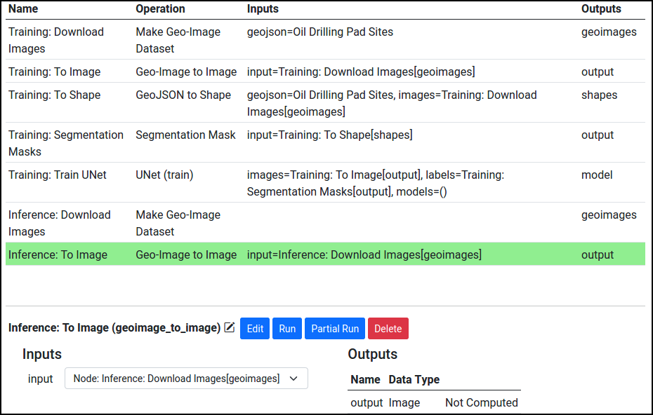
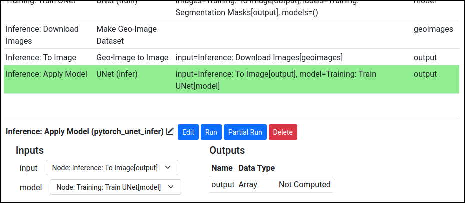
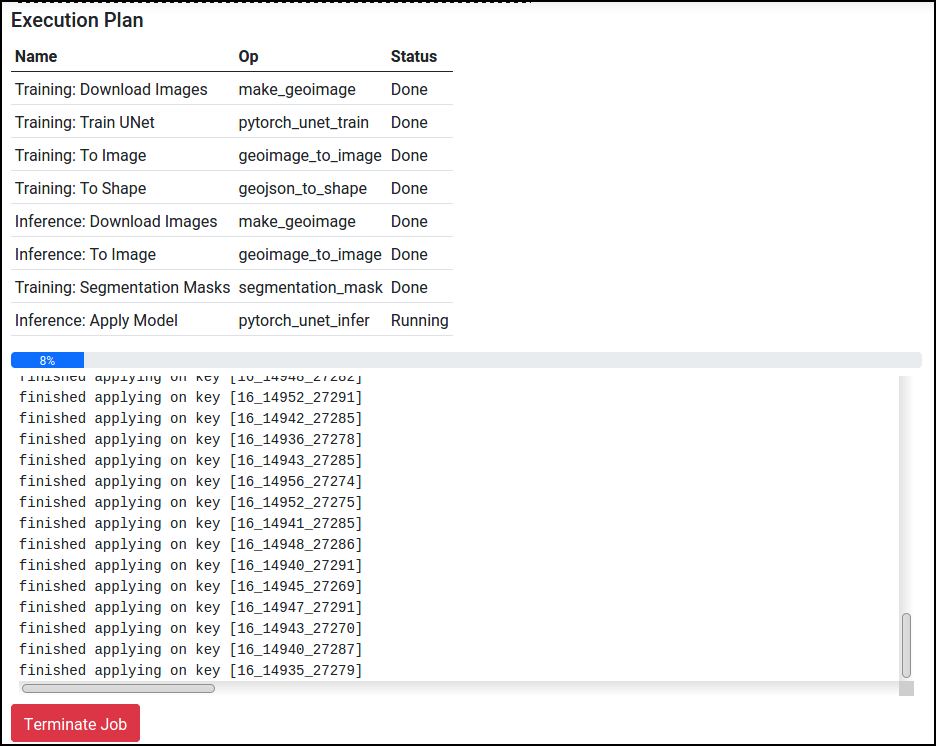
We can now add a UNet (infer) operation to apply the trained model.

Post-processing

Lastly, we need to post-process the outputs of our segmentation model back into GeoJSON features (longitude-latitude coordinates) in order for them to be useful. SkyhookML includes operations for extracting polygon shapes from segmentation outputs, and for converting those shapes back into GeoJSON features.

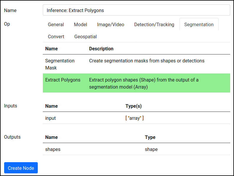
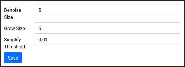
To extract polygons, add an Extract Polygons operation (from Segmentation tab). This model exposes parameters that control thinning/growing during polygon extraction, but the defaults usually work fine. Make sure to configure the operation to input the segmentation model outputs.

Then, add a Shape to GeoJSON operation to convert the shapes, which are polygons in pixel coordinates, to GeoJSON features, which are in longitude-latitude coordinates. The final, complete pipeline should look like this:

And that's it! After running the "Inference: To GeoJSON" node, we can visualize the GeoJSON data.